7 Command-Line Tools for Data Science

Sep 19, 2013 • 21 min read.
Data science is OSEMN (pronounced as awesome). That is, it involves Obtaining, Scrubbing, Exploring, Modelling, and iNterpreting data. As a data scientist, I spend quite a bit of time on the command-line, especially when there’s data to be obtained, scrubbed, or explored. And I’m not alone in this. Recently, Greg Reda discussed how the classics (e.g., head, cut, grep, sed, and awk) can be used for data science. Prior to that, Seth Brown discussed how to perform basic exploratory data analysis in Unix.
I would like to continue this discussion by sharing seven command-line
tools that I have found useful in my day-to-day work. The tools are:
jq,
json2csv,
csvkit, scrape,
xml2json, sample, and Rio. (The
home-made tools scrape, sample, and Rio can be found in this
repository.)
Any suggestions, questions, comments, and even pull requests are more
than welcome. (Tools suggested by others can be found towards the bottom
of the post.) OSEMN, let’s get started with our first tool: jq.
1. jq - sed for JSON
JSON is becoming an increasingly common data format, especially as APIs
are appearing everywhere. I remember cooking up the ugliest grep and
sed incantations in order to process JSON. Thanks to jq, those days
are now in the past.
Imagine we’re interested in the candidate totals of the 2008
presidential election. It so happens that the New York Times has a
Campaign Finance
API. (You can
get your own API keys if you
want to access any of their APIs.) Let’s get some JSON using curl:
$ curl -s 'http://api.nytimes.com/svc/elections/us/v3/finances/2008/president/totals.json?api-key=super-secret' > nyt.jsonwhere -s puts curl in silent mode. In its simplest form, i.e.,
jq '.', the tool transforms the incomprehensible API response we got:
$ cat nyt.json
{"status":"OK","base_uri":"http://api.nytimes.com/svc/elections/us/v3/finances/2008/","cycle":2008,"copyright":"Copyright (c) 2013 The New York Times Company. All Rights Reserved.","results":[{"candidate_name":"Obama, Barack","name":"Barack Obama","party":"D", ...
into nicely indented output:
$ < nyt.json jq '.' | head
{
  "results": [
    {
      "candidate_id": "P80003338",
      "date_coverage_from": "2007-01-01",
      "date_coverage_to": "2008-11-24",
      "candidate_name": "Obama, Barack",
      "name": "Barack Obama",
      "party": "D",
Note that the output isn’t necessarily in the same order as the input.
Besides pretty printing, jq can also select, filter, and format JSON
data, as illustrated by the following command, which returns the name,
cash, and party of each candidate that had at least $1,000,000 in cash:
$ < nyt.json jq -c '.results[] | {name, party, cash: .cash_on_hand} | select(.cash | tonumber > 1000000)'
{"cash":"29911984.0","party":"D","name":"Barack Obama"}
{"cash":"32812513.75","party":"R","name":"John McCain"}
{"cash":"4428347.5","party":"D","name":"John Edwards"}
Please refer to the jq manual to
read about the many other things it can do, but don’t expect it to solve
all your data munging problems. Remember, the Unix philosophy favours
small programs that do one thing and do it well. And jq’s
functionality is more than sufficient I would say! Now that we have the
data we need, it’s time to move on to our second tool: json2csv.
2. json2csv - convert JSON to CSV
While JSON is a great format for interchanging data, it’s rather
unsuitable for most command-line tools. Not to worry, we can easily
convert JSON into CSV using
json2csv. Assuming that we stored
the data from the last step in million.json, simply invoking
json2csv will convert it to some nicely comma-separated values:
$ < million.json json2csv -k name,party,cash | head -n 3
Barack Obama,D,29911984.0
John McCain,R,32812513.75
John Edwards,D,4428347.5
Having the data in CSV format allows us to use the classic tools such as
cut -d, and awk -F,. Others like grep and sed don’t really have
a notion of fields. Since CSV is the king of tabular file formats,
according to the authors of csvkit,
they created, well, csvkit.
3. csvkit - suite of utilities for working with CSV
Rather than being one tool, csvkit is
a collection of tools that operate on CSV data. Most of these tools
expect the CSV data to have a header, so let’s add one. (Since the
publication of this post, json2csv has been updated to print the
header with the -p option.)
$ echo name,party,cash | cat - million.csv > million-header.csvWe can, for example, sort the candidates by cash with csvsort and
display the data using csvlook:
$ < million-header.csv csvsort -rc cash | csvlook
|---------------+-------+--------------|
|  name         | party | cash         |
|---------------+-------+--------------|
|  John McCain  | R     | 32812513.75  |
|  Barack Obama | D     | 29911984.0   |
|  John Edwards | D     | 4428347.5    |
|---------------+-------+--------------|
Looks like the MySQL console doesn’t it? Speaking of databases, you can insert the CSV data into an sqlite database as follows (many other databases are supported as well):
$ csvsql --db sqlite:///myfirst.db --insert million-header.csv
$ sqlite3 myfirst.db
sqlite> .schema million-header
CREATE TABLE "million-header" (
    name VARCHAR(12) NOT NULL,
    party VARCHAR(1) NOT NULL,
    cash FLOAT NOT NULL
);
In this case, the database columns have the correct data types because
the type is inferred from the CSV data. Other tools within csvkit that
might be of interest are: in2csv, csvgrep, and csvjoin. And with
csvjson, the data can even be converted back to JSON. All in all,
csvkit is worth checking out.
4. scrape - HTML extraction using XPath or CSS selectors
JSON APIs sure are nice, but they aren’t the only source of data; a lot
of it is unfortunately
still
embedded in HTML.
scrape is a
python script I put together that employs the lxml and cssselect
packages to select certain HTML elements by means of an XPath query or
CSS
selector.
Let’s extract the table from this Wikipedia article that lists the
border and area ratio of each
country.
$ curl -s 'http://en.wikipedia.org/wiki/List_of_countries_and_territories_by_border/area_ratio' |
> scrape -b -e 'table.wikitable > tr:not(:first-child)' | head
<!DOCTYPE html>
<html>
<body>
<tr>
<td>1</td>
<td>Vatican City</td>
<td>3.2</td>
<td>0.44</td>
<td>7.2727273</td>
</tr>
The -b argument lets scrape enclose the output with <html> and
<body> tags, which is sometimes required by xml2json to convert
correctly the HTML to JSON.
5. xml2json - convert XML to JSON
As its name implies, xml2json
takes XML (and HTML) as input and returns JSON as output. Therefore,
xml2json is a great liaison between scrape and jq.
$ curl -s 'http://en.wikipedia.org/wiki/List_of_countries_and_territories_by_border/area_ratio' |
> scrape -be 'table.wikitable > tr:not(:first-child)' |
> xml2json |
> jq -c '.html.body.tr[] | {country: .td[1][], border: .td[2][], surface: .td[3][], ratio: .td[4][]}' | head
{"ratio":"7.2727273","surface":"0.44","border":"3.2","country":"Vatican City"}
{"ratio":"2.2000000","surface":"2","border":"4.4","country":"Monaco"}
{"ratio":"0.6393443","surface":"61","border":"39","country":"San Marino"}
{"ratio":"0.4750000","surface":"160","border":"76","country":"Liechtenstein"}
{"ratio":"0.3000000","surface":"34","border":"10.2","country":"Sint Maarten (Netherlands)"}
{"ratio":"0.2570513","surface":"468","border":"120.3","country":"Andorra"}
{"ratio":"0.2000000","surface":"6","border":"1.2","country":"Gibraltar (United Kingdom)"}
{"ratio":"0.1888889","surface":"54","border":"10.2","country":"Saint Martin (France)"}
{"ratio":"0.1388244","surface":"2586","border":"359","country":"Luxembourg"}
{"ratio":"0.0749196","surface":"6220","border":"466","country":"Palestinian territories"}
Of course this JSON data could then be piped into json2csv and so
forth.
6. sample - when you’re in debug mode
The second tool I made is
sample.
(It’s based on two scripts in bitly’s
data_hacks, which contains some
other tools worth checking out.) When you’re in the process of
formulating your data pipeline and you have a lot of data, then
debugging your pipeline can be cumbersome. In that case, sample might
be useful. The tool serves three purposes (which isn’t very Unix-minded,
but since it’s mostly useful when you’re in debug mode, that’s not such
a big deal).
The first purpose of sample is to get a subset of the data by
outputting only a certain percentage of the input on a line-by-line
basis. The second purpose is to add some delay to the output. This comes
in handy when the input is a constant stream (e.g., the Twitter
firehose), and the data comes in too fast to see what’s going on. The
third purpose is to run only for a certain time. The following
invocation illustrates all three purposes.
$ seq 10000 | sample -r 20% -d 1000 -s 5 | jq '{number: .}'This way, every input line has a 20% chance of being forwarded to jq.
Moreover, there is a 1000 millisecond delay between each line and after
five seconds sample will stop entirely. Please note that each argument
is optional. In order to prevent unnecessary computation, try to put
sample as early as possible in your pipeline (the same argument holds
for head and tail). Once you’re done debugging you can simply take
it out of the pipeline.
7. Rio - making R part of the pipeline
This post wouldn’t be complete without some R. It’s not straightforward to make R/Rscript part of the pipeline since they don’t work with stdin and stdout out of the box. Therefore, as a proof of concept, I put together a bash script called Rio.
Rio works as follows. First, the CSV provided to stdin is redirected
to a temporary file and lets R read that into a data frame df. Second,
the specified commands in the -e option are executed. Third, the
output of the last command is redirected to stdout. Allow me to
demonstrate three one-liners that use the Iris dataset (don’t mind the
url).
Display the five-number-summary of each field.
$ curl -s 'https://raw.github.com/pydata/pandas/master/pandas/tests/data/iris.csv' > iris.csv
$ < iris.csv Rio -e 'summary(df)'
  SepalLength      SepalWidth     PetalLength      PetalWidth
 Min.   :4.300   Min.   :2.000   Min.   :1.000   Min.   :0.100
 1st Qu.:5.100   1st Qu.:2.800   1st Qu.:1.600   1st Qu.:0.300
 Median :5.800   Median :3.000   Median :4.350   Median :1.300
 Mean   :5.843   Mean   :3.054   Mean   :3.759   Mean   :1.199
 3rd Qu.:6.400   3rd Qu.:3.300   3rd Qu.:5.100   3rd Qu.:1.800
 Max.   :7.900   Max.   :4.400   Max.   :6.900   Max.   :2.500
     Name
 Length:150
 Class :character
 Mode  :character
If you specify the -s option, the sqldf package will be imported. In
case the output is a data frame, CSV will be written to stdout. This
enables you to further process that data using other tools.
$ < iris.csv Rio -se 'sqldf("select * from df where df.SepalLength > 7.5")' | csvlook
|--------------+------------+-------------+------------+-----------------|
|  SepalLength | SepalWidth | PetalLength | PetalWidth | Name            |
|--------------+------------+-------------+------------+-----------------|
|  7.6         | 3          | 6.6         | 2.1        | Iris-virginica  |
|  7.7         | 3.8        | 6.7         | 2.2        | Iris-virginica  |
|  7.7         | 2.6        | 6.9         | 2.3        | Iris-virginica  |
|  7.7         | 2.8        | 6.7         | 2          | Iris-virginica  |
|  7.9         | 3.8        | 6.4         | 2          | Iris-virginica  |
|  7.7         | 3          | 6.1         | 2.3        | Iris-virginica  |
|--------------+------------+-------------+------------+-----------------|
If you specify the -g option, ggplot2 gets imported and a ggplot
object called g with df as the data is initialised. If the final
output is a ggplot object, a PNG will be written to stdout.
$ < iris.csv Rio -ge 'g + geom_point(aes(x = SepalLength, y = SepalWidth, colour = Name))' > iris.png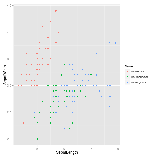
I made this tool so that I could take advantage of the power of R on the command-line. Of course it has its limits, but at least there’s no need to learn gnuplot any more.
Command-line tools suggested by others
Below is an uncurated list of tools and repositories that others have suggested via Twitter or Hacker News (last updated on 23-09-2013 07:15 EST). Thanks everybody.
- BigMLer by aficionado
- crush-tools by mjn
- csv2sqlite by dergachev
- csvquote by susi22
- data-tools repository by cgrubb
- feedgnuplot by dima55
- Grinder repository by @cgutteridge
- HDF5 Tools by susi22
- littler by @eddelbuettel
- mallet by gibrown
- RecordStream by revertts
- subsample by paulgb
- xls2csv by @sheeshee
- XMLStarlet by gav
Conclusion
I have shown you seven command-line tools that I use in my daily work as
a data scientist. While each tool is useful in its own way, I often find
myself combining them with, or just resorting to, the classics such as
grep, sed, and awk. Combining such small tools into a larger
pipeline is what makes them really powerful.
I’m curious to hear what you think about this list and what command-line tools you like to use. Also, if you’ve made any tools yourself, you’re more than welcome to add them to this data science toolbox.
Don’t worry if you don’t regard yourself as a toolmaker. The next time
you’re cooking up that exotic pipeline, consider to put it in a file,
add a shebang,
parametrise it with some $1s and $2s, and chmod +x it. That’s all
there is to it. Who knows, you might even become interested in applying
the Unix philosophy.
While the power of the command-line should not be underestimated when it comes to Obtaining, Scrubbing, and Exploring data, it can only get you so far. When you’re ready to do some more serious Exploring, Modelling, and iNterpretation of your data, you’re probably better off continuing your work in a statistical computing environment, such as R or Jupyter Notebook+pandas.
— Jeroen
Would you like to receive an email whenever I have a new blog post, organize an event, or have an important announcement to make? Sign up to my newsletter: